Frequentist vs Bayesian

Frequentist: Long term relative Frequency

• $\Theta$ are a set of unkonw constraings
• Observed data
• Follows a sampling distribution

Bayesian: A degree of subjective belief

• $\theta$ are random variables
• Combine with prior belifs
• Follows Posterior Distribution

Frequentist Estimation

Estimators: MLE, Method of Moments Solving for $\theta$ gives the MLE estimator: ${\hat{\theta }}_{MLE}=\frac{x}{n}$

• $x$ is the number of occurrences
• $n$ total data

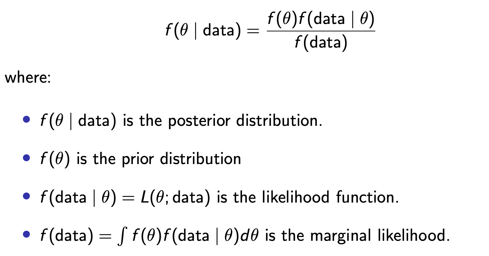
Bayesian Estimation

Model parameters are expressed as $\theta$ through prior distribution.

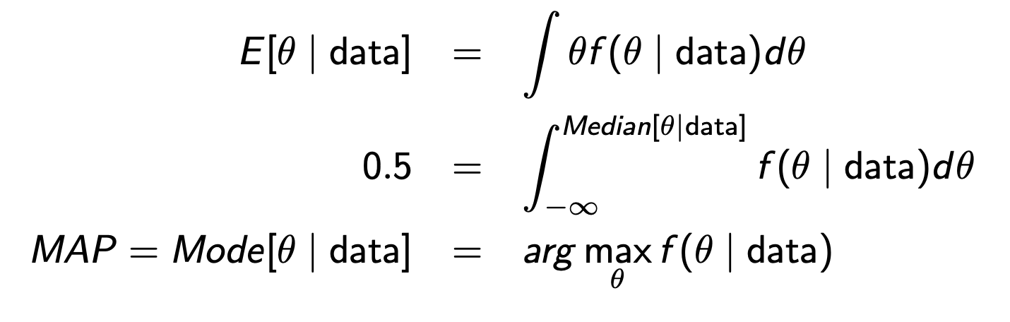
Point Estimation

Questions:

1. Assume a beta prior distribution, B(5,5), for the probability of head. Suppose we toss the coin 12 times and observe 9 heads and 3 tails. Obtain the posterior mean, median and mode. Compare with the MLE estimation.

alpha = 5
beta = 5
 
n = 12
heads = 9
tails = 3
alpha_post = integer(alpha) + 9
beta_post = integer(beta) + tails
 
 
post_mean   <- alpha_post / (alpha_post + beta_post)
post_median <- qbeta(0.5, alpha_post, beta_post)
post_map    <- (alpha_post - 1) / (alpha_post + beta_post - 2)
cat("mean", post_mean, "median", post_median, "mode", post_map)

mean 0.75, median 0.7642145 mode 0.8 2. Read the file sms.csv. Asuming a B(5,5) prior and given 5000 data, obtain the posterior mean, median and mode. Compare with the MLE estimation.

alpha = 5
beta = 5
data = sms
alpha_post = alpha + sum(data$type == 'spam')
beta_post = beta + (nrow(data) - sum(data$type == 'spam'))
post_mean   <- alpha_post / (alpha_post + beta_post)
post_median <- qbeta(0.5, alpha_post, beta_post)
post_map    <- (alpha_post - 1) / (alpha_post + beta_post - 2)
mle = sum(data$type == 'spam') / nrow(data)
cat("MLE Estimation",mle ,"\nmean", post_mean, "median", post_median, "mode", post_map)
 

MLE Estimation 0.1343767 mean 0.1350332 median 0.1349895 mode 0.1349021

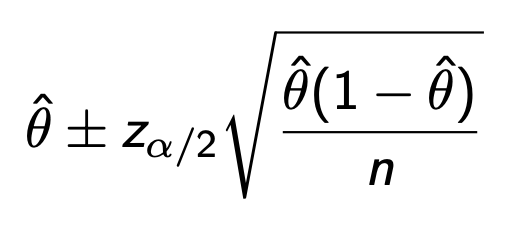
Frequentist Confidence Intervals

$1-a$ confidence interval for $\theta$ and is represented as repetitions of Random Experiments

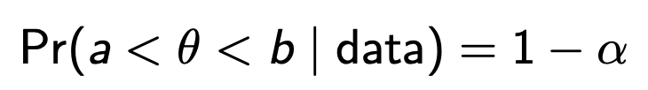
Bayesian Confidence Intervals

Based on prior: Bayesian credible intervals are based on the posterior distribution. A $(1-\alpha )$ credible interval is any interval (a,b) such that:

Questions: Assume a beta prior distribution, B(5,5), for the probability of head. Suppose we toss the coin 12 times and observe 9 heads and 3 tails. Obtain a 95% credible interval for the probability of head. Compare with frequentist intervals of the previous example.

alpha = 5
beta = 5
n = 12
heads = 9
tails = 3
 
# Bayesian Approach
alpha_post = heads + alpha
beta_post = tails + beta
 
confidence_interval = qbeta(c(0.025, 0.975), alpha_post, beta_post)
 
#Frequentist Approach
test = binom.test(heads, n, conf.level = 0.95)
confidence_interval_f = test$conf.int
cat("Bayesian Approach", confidence_interval, "\nFrequentist Approach", confidence_interval_f)

Bayesian Approach 0.4303245 0.8189284 Frequentist Approach 0.4281415 0.9451394

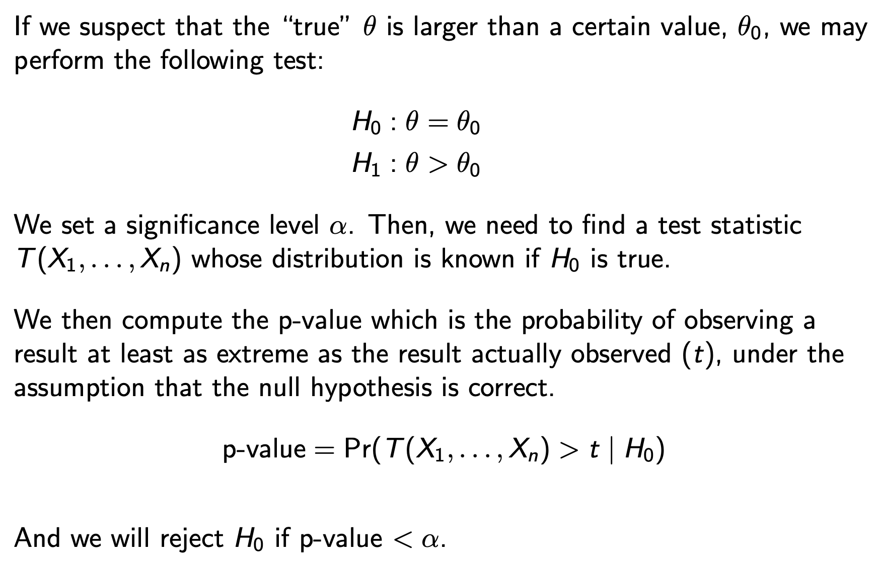
Frequentist Hypothesis Testing:

Bayesian Hypothesis Testing

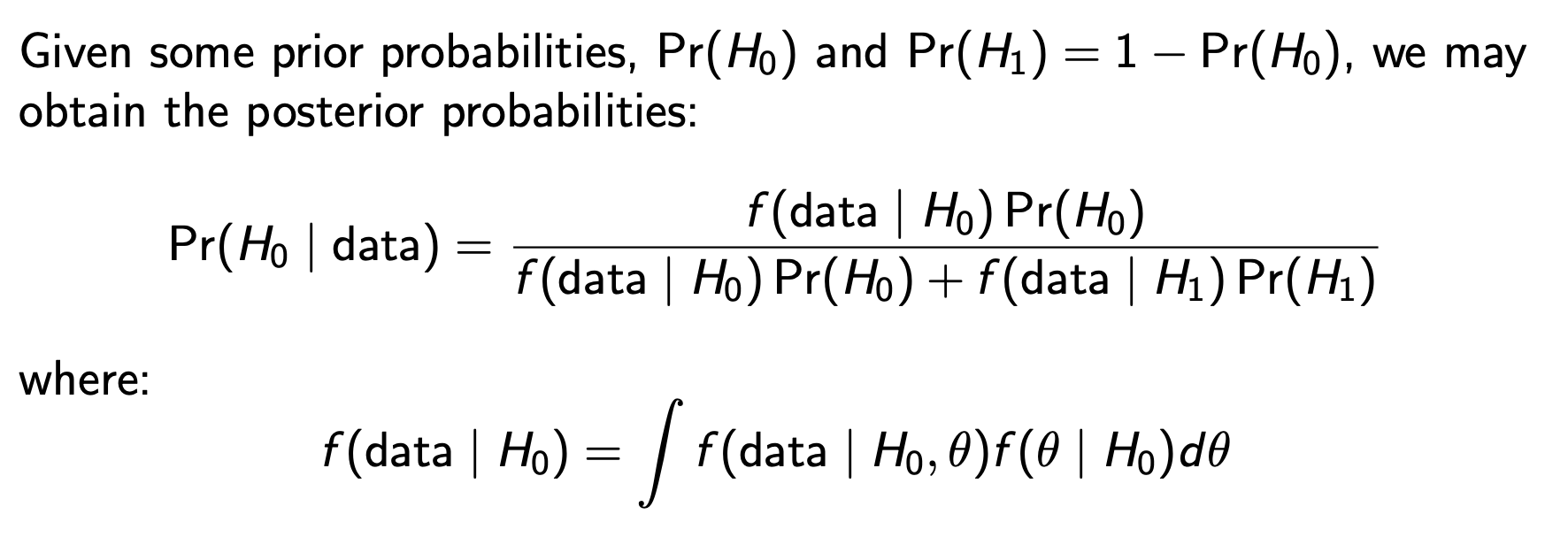
Questions: Assume a beta prior distribution, B(5,5), for the probability of head. Suppose we toss the coin 12 times and observe 9 heads and 3 tails. Test the null hypothesis, H0 : θ≤0.5 against the alternative H1 : θ>0.5. Compare with frequentist results

alpha_prior <- 5
beta_prior <- 5
freq_test <- binom.test(x, n, p = 0.1, alternative = "greater")
alpha_post <- alpha_prior + x
beta_post  <- beta_prior + (n - x)
 
prob_H1 <- 1 - pbeta(0.1, alpha_post, beta_post)
prob_H0 <- pbeta(0.1, alpha_post, beta_post)
 

--- Frequentist Results --- P-value: 1e-12 Conclusion: Reject H0

--- Bayesian Results --- P(H0 | Data): 0 P(H1 | Data): 1 Conclusion: The probability that theta > 0.1 is 100 %

The Predictive Distribution Frequentist

The predictive distribution is expressed as: $p(x_{new}\mid \hat{\theta })$

Parameter Uncertainty

This method does not fully account for parameter uncertainty. It treats the estimate $\hat{\theta }$ as the “absolute truth,” ignoring the fact that a different sample could have yielded a different $\hat{\theta }$.

Bayesian Prediction: The Posterior Predictive Distribution

From the Bayesian point of view, prediction is handled by averaging over all possible values of $\theta$, weighted by their posterior probability. This is known as the predictive distribution:

$f(x_{new}\mid \text{data})=\int f(x_{new}\mid \theta )f(\theta \mid \text{data})d\theta$

Question: Suppose we toss a coin 12 times and observe 9 heads and 3 tails. Predict the probability that in the next 12 tosses you observe exactly 9 heads.

p_hat <- 9 / 12
freq_pred <- dbinom(9, size = 12, prob = p_hat)
cat("Frequentist Prediction:", round(freq_pred, 4))
 
# Bayesian Predictions
alpha_post <- 5 + 9  
beta_post  <- 5 + 3  
predictive_func <- function(p) {
  dbinom(9, size = 12, prob = p) * dbeta(p, alpha_post, beta_post)
}
bayesian_pred <- integrate(predictive_func, 0, 1)$value
cat("Bayesian Prediction:", round(bayesian_pred, 4))

Frequentist Prediction: 0.2581 Bayesian Prediction: 0.1682

publish